Time Complexity of an Algorithm

What is the Best Way to Compare Algorithms' Efficiency?

Given two algorithms that perform the same task, what is the best way to compare their performance? At first glance, one might consider measuring the runtime of the two algorithms. However, this is not a reliable metric, as runtime depends heavily on the hardware and can be highly inconsistent due to real-world conditions, even on the same machine. To address this problem, scientists have developed a more theoretical approach called the time complexity of an algorithm. This measure evaluates how an algorithm's performance scales as the size of the input increases.

If $n$ is the number of input, then for a given algorithm, there exists a function $f(n)$ that measures the worst-case runtime of the algorithm as $n$ varies. The runtime of an algorithm generally follows a specific trend, such as constant, logarithmic, or linear. However, as noted, the runtime is significantly influenced by hardware and physical conditions. Therefore, these functions are often expressed with additional constant factors, such as:

where $C_1$ and $C_0$ are factors that depends on outside conditions. This expression is quite inconvenient, as we don't usually know what these constant factors are, so the general rule of thumb to express the worst-case runtime of an algorithm is through the big-O notation. For $f(n) = C_1n + C_0$, for example, if $f(n) = C_1n + C_0$, then $f(n)$ it can be said that

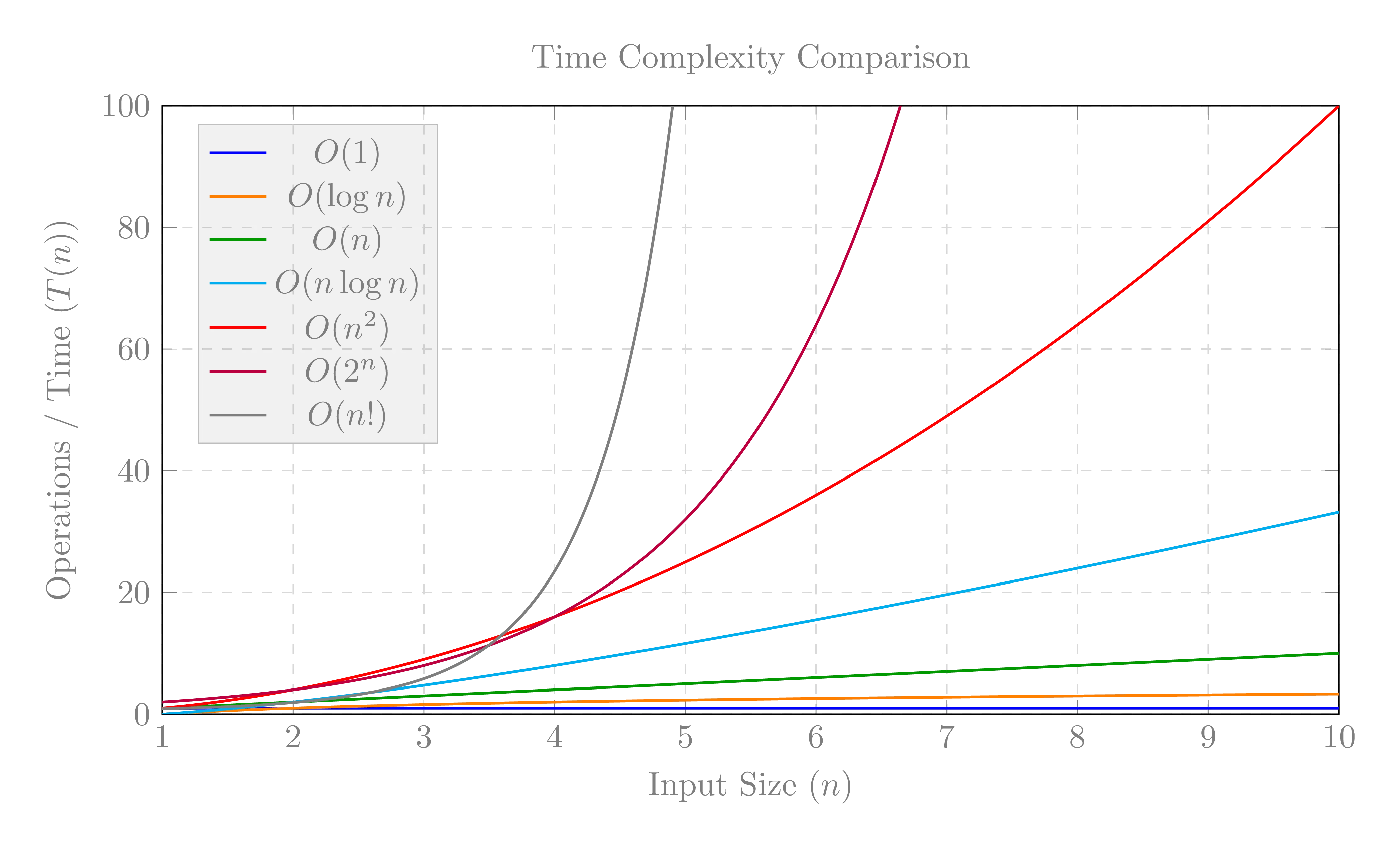
There are many categories of such functions $f(n)$, and the most important functions used in algorithmic analysis are the constant function, $f(n)=c$, the logarithm function $f(n) = \log_b(n)$, the linear function $f(n) = n$, $f(n) = n\log(n)$, the quadratic function $f(n) = n^2$, other polynomial functions $f(n) = n^d$, the exponential functions $f(n) = a^n$, and the factorial function $f(n) = n!$.

The Big O, Big Omega, Big Theta, and Their Properties

Algorithmic Analysis

How can we determine the time complexity of an algorithm? Consider the following example: finding the largest element in an array.

    // Algorithm: find the maximum element of an array of integers
    // Input: an array A of size n
    // Output: maximum element of A
    array_max(int A[], int n){
        int current_max = A[0];
        for (i = 1 ; i < n; i++)
            if (A[i] > current_max)
                current_max = A[i];
        return current_max;
     } 

The assignment operator current_max = A[0] takes constant time, $f(n)=c$. In the for loop, the operator i = 1 also takes constant time, $f(n)=c$. The comparison operator, also takes constant time, but the operator repeated $n$ times, so the runtime function is $f(n) = c_1n + c_0$.

The constant function

The constant time complexity function, denoted

does not depend on the size of the input (unless the size of the input is exceptionally large). Some examples of algorithms with this complexity are:

• Accessing array index: Accessing elements at a specific index in an array takes constant time because an array begins at a fixed memory location. The memory location of each element can be directly calculated using the element's size and its index, which is a constant operation.

• Basic arithmetic and bitwise operations: Computers usually uses 8-bit, 16-bit, 32-bit, and 64-bit for integers and floating point numbers. Addition, subtraction, multiplication, or division of two numbers are considered constant time complexity because they are limited to a certain amount of bit. However, for large number arithmetic with arbitrary precision, the time complexity will no longer be constant.

  Bitwise operations like AND, OR, and XOR also take constant time because, again, primitive data types are limited to a certain size on the computer.

• Variable assignment: For primitive data types such as integers, floating points, characters, and boolean, the assignment operator takes constant time complexity because the size of these variables are pre-determined. However, for non-primitive data types such as strings, the assignment operator takes linear time, $O(n)$ because strings are arrays of characters.
• Returning a value from a function: Returning a pre-defined value also takes constant time.
• Inserting a node, or jump to the next/previous node in a linked list: These operation are constant because each node holds the address of the next node (for a singly linked list), or the address of both the previous and the next node (for a doubly linked list).
• Pushing and popping on stack. Insertion and removal from queue.
• Hashmap operations: Insert, access, and search operations in a hash map take constant time on average (ideally). These operations are $O(1)$ on average because a hash map uses a bucket array, and accessing elements in an array is $O(1)$. The hash function computes an index for a given key, and ideally, keys are distributed evenly across the buckets. However, if all keys end up in the same bucket due to hash collisions (e.g., in separate chaining), these operations degrade to $O(n)$ in the worst case, where $n$ is the total number of keys in the hash map.

The Logarithm Function

Some examples of this type of algorithms are:

• Binary search: binary search involves searching for an element in a sorted array. This algorithm is $O(\log n)$ because it utilizes the divide and conquer technique, where the size of the array reduces by half every iteration.
• Calculate the 64-bit (or less) $n$-th Fibinacci number with fast doubling method.
• Balanced Binary Search Trees (e.g., AVL Tree, Red-Black Tree): Searching, insertion, and deletion in balanced binary search trees like AVL trees, Red-Black trees, or B-trees operate in $O(\log n)$ because the height of a balanced tree is $O(\log n)$.
• Binary Heap Operations: Operations like insertion and extracting the minimum (or maximum) in a binary heap take $O(\log n)$ time because of heapify operations.
• Exponentiation by Squaring: This algorithm utilizes the divide and conquer method by checking whether $n$ is even or odd.

      Input: a real number x; an integer n
      Output: x^n
      exp_by_squaring(x, n)
          if n < 0 then
              return exp_by_squaring(1 / x, -n);
          else if n = 0 then 
              return 1;
          else if n is even then 
              return exp_by_squaring(x * x, n / 2);
          else if n is odd then 
              return x * exp_by_squaring(x * x, (n - 1) / 2);
      end function 

• Finding the Greatest Common Divisor (GCD)

The Linear Function

• Finding the maximum/minimum of an array: We can only find the maximum or the minimum of an array by going over all elements of the array.
• Linear search: If the elements are not sorted, then to find an element in an array, we must perform linear search, which has the worst-case complexity of $O(n)$. Similarly, traversing a linked list is also $O(n)$.
• Deletion and Insertion at random position in a linked list or array. This tasks requires us to traverse over each individual elements/nodes, which has the worst-case complexity of $O(n)$.
• Comparing arrays, linked list, strings.

The $n \log n$ Function

These types of algorithms are usually optimized versions of $O(n^2)$ algorithms. Some examples of this type of algorithms are:

• Fast Fourier Transform: FFT works by breaking down the computation of the Discrete Fourier Transform (DFT), which is $O(n^2)$ nto smaller subproblems. For an input signal of size $n$, the FFT algorithm splits it into two halves: one for the even-indexed terms and one for the odd-indexed terms. It then recursively computes the DFT of these smaller subproblems: the even and odd indexes terms of the DFT.
• Merge Sort, Quick Sort (on average), Heap Sort, AVL Tree Sort are all $O(n\;\log n)$ algorithms.

The Exponential Function

Algorithms of this type are generally very bad. Some examples are:

• Subset Sum Problem (Brute Force): Given a set of integers, determine if there is a subset whose sum equals a given target value. A brute-force approach would involve checking every possible subset of the set to see if its sum equals the target. Time Complexity: $O(2^n)$ because there are
  $$S = \sum_{k=0}^{n}\binom{n}{k} = \binom{n}{1} + \binom{n}{2} + \ldots + \binom{n}{n} = 2^n.$$
  subsets of a set of $n$ elements.
• Naive Recursive Fibonacci: Compute the n-th Fibonacci number, where $F(n) = F(n-1) + F(n-2)$ and the base cases are $F(0) = 0$ and $F(1) = 1$. The time complexity of this problem is $O(2^n)$ because the recursive calls grow exponentially due to repeated subproblems.
• Find all sub-arrays of an array. This algorithm actually has an time complexity of $O(n\cdot 2^n)$ because the total number of non-empty sub-arrays in an array of size $n$ is $2^n - 1$ and we also need to loop over $n$ elements of the array.

The Factorial Function

• The Traveling Salesman Problem (TSP) - Brute Force Approach: Given a set of cities, find the shortest possible route that visits each city exactly once and returns to the origin city. A brute force approach checks all possible permutations of the cities to find the optimal solution.
• Generating Factorials: Given a set of integers $S=\{1, 2, \ldots, n\}$. Since there are up to $n!$ permutations of elements of this set, generating all possible permutation will requires $O(n!)$.