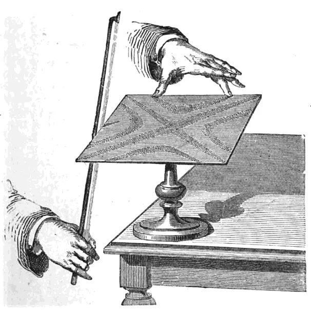
The general model and the boundary condition
Depends on whether you clamp your edge or not, clamp the edge
partially, or simply support the plate by placing some other objects
below the plate; the boundary condition may be different. For this
project, we will emphasize the free boundary condition. That is, only
the wave generator supports the plate.
| Type of Boundary | Boundary Condition |
| Clamped (fixed) edge | $u(\pm a, y, t) = u(x, \pm a, t) = 0$ |
| Moving edge | $u(a, y, t_0) = f(y, t)$ |
| Free edge |
$\pd{u}{x}(\pm a, y, t) =
\pd{u}{y}(x, \pm a, t) = 0$ |
The free boundary condition means that there are no forces acting on
the edges of the plate; that is, expressed mathematically,
\begin{equation} \pd{u}{x}(\pm a, y, t)
= \pd{u}{y}(x, \pm a, t) = 0
\end{equation}
which gave us four boundary conditions. The uniqueness of the solution
requires our equation to have two more initial conditions. Similar to
ordinary differential equations, these conditions are the initial
displacement and velocity of the plate at $t=0$. That is,
\begin{equation} u(x,y,0) = f(x,y)
\quad\text{and}\quad u_t(x,y,0) = g(x,y)
\end{equation}
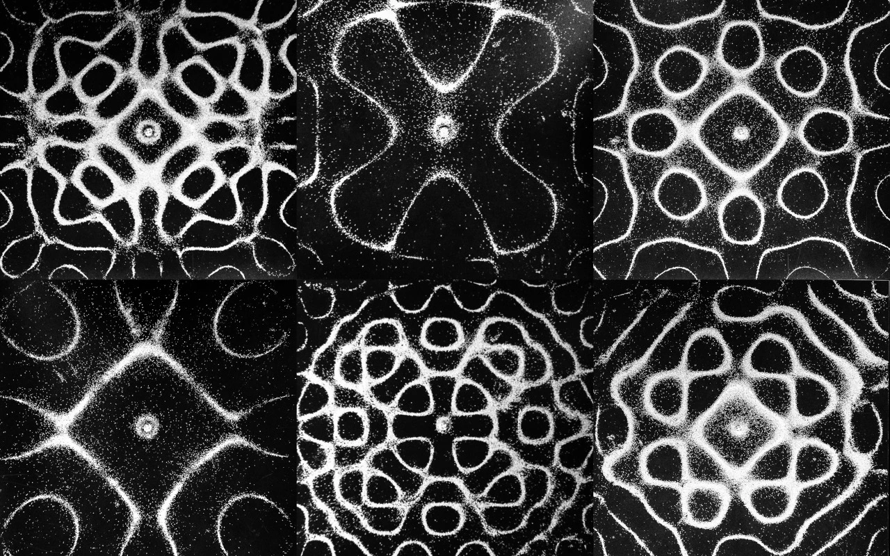
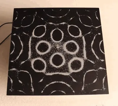
The Square Plate
Consider the wave equation on a rectangle $\Omega =
\{(x,y)\in\R^2\;|\; -a\leq x,y\leq a\}$,
\begin{equation} u_{tt} = c^2\nabla^2u + Q,\quad
\mathbf{x}\in\Omega \end{equation}
with boundary conditions
\begin{equation} u_x(\pm a, y, t) = u_y(x, \pm a, t) = 0
\end{equation}
and initial conditions
\begin{equation} u(x,y,0) = f(x,y), \quad\quad u_t(x,y,0)
= g(x,y). \end{equation}
Here, $a$ is half the length of the plate, and also note that we
denote the length of the plate to be $L$. A standard way to solve a
forced differential equation is to solve its homogenous case first,
i.e. when $Q=0$.There are many ways to solve this initial-boundary
value problem, and one common, and easy-to-understand technique is via
separation of variables. If we assume that $u$ is separable and let
$u(x,y,t) = X(x)Y(y)T(t)$, the equation becomes
\begin{equation} XYT'' = c^2(X''YT + XY''T)
\end{equation}
Divide both sides by $XYT$, we obtain
\begin{equation}
\frac{T''}{c^2T}=\frac{X''}{X}+\frac{Y''}{Y}=-\lambda
\end{equation}
Notice that
$\frac{X''}{X}+\frac{Y''}{Y}=-\lambda$
is constant if and only if $X''/X=-\mu$ and $Y''/Y = -\nu$, where
$\mu$ and $\nu$ are themselves constants and $\lambda = \mu + \nu$.
The two constants above yield two eigenvalue problems with Neumann
boundary conditions:
\begin{align} X''(x)+\mu X(x)&=0, \quad X'(-a)=X'(a)=0
\label{eq:X1}\\ Y''(y)+\nu Y(y)&=0, \quad Y'(-a)=Y'(a)=0
\label{eq:Y1}, \end{align}
and the time equation yields the third eigenvalue problem:
\begin{equation} T''(t) + c\lambda^2T(t) = 0
\end{equation}
The detail solution of these eigenvalue problems is beyond the scope
of this article. For the detail solution, again, please refer to my project report. The general idea is we need to solve the eigenvalue problems
(\ref{eq:X1}) and (\ref{eq:Y1}) first, and from
there we solve the third eigenvalue problem, since $\lambda = \mu +
\nu$. After carrying out all the hard work, the eigenvalues for
equations (\ref{eq:X1}) and (\ref{eq:Y1}) are
\begin{equation} \mu =
\left(\frac{n\pi}{2a}\right)^2 =
\left(\frac{n\pi}{L}\right)^2, \quad \nu =
\left(\frac{m\pi}{2a}\right)^2 =
\left(\frac{m\pi}{L}\right)^2
\end{equation}
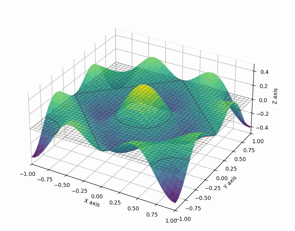
and the solution to the homogeneous equation is the double Fourier
series
\begin{equation} u(x,y,t) =
\frac{1}{4}A_{00} +
\sum_{n=1}^{\infty}\sum_{m=1}^{\infty}X_n(x)Y_n(y)T_{nm}(t)
\end{equation}
where,
\begin{align} X_n(x) &= a_n\cos\left(\frac{n\pi
x}{L}\right) +
\overline{a_n}\sin\left(\frac{n\pi
x}{L}\right)\\[0.5em] Y_m(y) &=
a_m\cos\left(\frac{m\pi y}{L}\right) +
\overline{a_m}\sin\left(\frac{m\pi
y}{L}\right)\\[0.5em] T_{nm}(t) &=
A_{nm}\cos(\omega t) + B_{nm}\sin(\omega
t)\\[0.5em] \omega &=
\frac{\pi}{L}c\sqrt{n^2+m^2}.
\end{align}
The coefficients $a_n$ and $\overline{a_n}$ are defined as
$a_n = \frac{1 +
(-1)^n}{2},\overline{a_n} = \frac{1 -
(-1)^n}{2}$, and,
\begin{alignat}{2} A_{nm} &=
\frac{4}{L^2}\int_{-L/2}^{L/2}\int_{-L/2}^{L/2}
f(x, y)X_n(x)Y_m(y)\;dxdy,\quad && n, m= 0, 1, 2,\ldots\\
B_{nm} &= \frac{4}{L^2}
\int_{-L/2}^{L/2}\int_{-L/2}^{L/2}
\frac{g(x, y)}{\omega}X_n(x)Y_m(y)\;dxdy,\quad
&& n, m= 1, 2, 3\ldots \end{alignat}
The forcing term $Q$ doesn't change the overall shape of the patterns,
but it does change the displacement of the plate overtime, hence the
time function $T_{nm}(t)$ becomes
\begin{equation} W_{nm}(t) =
A_{nm}\cos(\omega t) + B_{nm}\sin(\omega t) +
\int_{0}^{t}q_{nm}(\tau)\frac{\sin(\omega
t-\omega\tau)}{\omega}d\tau \end{equation}
Here, $q_{nm}$ is a function defined on the disk of radius
$r$ — the radius of the tip of the wave generator,
\begin{equation}
q_{nm}(\tau)=\frac{4\alpha}{L^2}
\cos(\omega_0 \tau) \iint_{U(r)}X_n(x)Y_m(y)\;dx dy,\quad
U(r)=\{(x,y)\in\R^2\;|\; x^2+y^2\leq r^2\}
\end{equation}
The Circular Plate
Consider the polar wave equation on a disk $\Omega =
\{(r,\theta)\in\R^2\;|\; 0 \leq r\leq a, 0 \leq \theta\leq
2\pi\},$
\begin{equation}
\secondpd{u}{t}=c^2\left(\secondpd{u}{r}+\frac{1}{r}\pd{u}{r}+\frac{1}{r^2}\secondpd{u}{\theta}\right)
+ Q(r, \theta, t). \end{equation}
Written in compact form with full boundary conditions:
\begin{equation} \begin{cases} u_{tt}
= c^2\lbrac u_{rr} + \dfrac{1}{r}u_r +
\dfrac{1}{r^2}u_{\theta\theta}\rbrac +
Q, & (r,\theta)\in\Omega\\ u_r(a,\theta, t) = 0\\[0.5em]
u(r,\theta, 0) = f(r, \theta)\\[0.5em] u_t(r, \theta, 0) = g(r,
\theta) \end{cases} \end{equation}
Let $u(r, \theta, t) = R(r)\Theta(\theta)T(t)$. Skipping all the hard work., we may arrive at the final solution to be
\begin{equation} u(r,\theta, t) =
\sum_{n=0}^{\infty}\sum_{m=0}^{\infty}J_n\lbrac
kr\rbrac[\Psi_{nm}(\theta)y_1(t) +
\Phi_{nm}(\theta)y_2(t)], \end{equation}
where
\begin{align} \Psi_{nm}(\theta) & =
a_{nm}\cos(n\theta) + b_{nm}\sin(n\theta)\\
\Phi_{nm}(\theta) &= c_{nm}\cos(n\theta) +
d_{nm}\sin(n\theta)\\ y_1(t) &= \alpha\cos(\omega t) +
\beta\sin(\omega t) +
\int_{0}^{t}p_{nm}(\tau)\frac{\sin(\omega(t-\tau))}{\omega}d\tau\\
y_2(t) &= \gamma\cos(\omega t) + \sigma\sin(\omega t) +
\int_{0}^{t}q_{nm}(\tau)\frac{\sin(\omega(t-\tau))}{\omega}d\tau\\
\omega &= \frac{cz_{nm}}{a} = ck.
\end{align}
Here, $z_{nm}$ are the zeros of the m-th derivative of the n-th
order Bessel function $J_n(x)$. $\alpha, \beta, \gamma, \sigma$ are arbitrary
constants that satisfies $\alpha + \gamma = 1,$ $\beta + \sigma = 1$, where
$\alpha^2 + \gamma^2 \neq 0$, $\beta^2 + \sigma^2 \neq 0$, and,
\begin{align} a_{nm} &= \frac{\langle
J_0\cos(n\theta), f \rangle_w}{\langle J_0, J_0
\rangle_w} =
\frac{\int_{0}^{a}\int_{0}^{2\pi}J_n\lbrac
kr\rbrac\cos(n\theta)
f(r,\theta)r\;drd\theta}{2\pi\int_{0}^{a}J_n^2\lbrac
kr\rbrac rdr},\quad n, m = 0, 1, \ldots\\ b_{nm}
&= \frac{\langle J_0\sin(n\theta), f
\rangle_w}{\langle J_0, J_0 \rangle_w} =
\frac{\int_{0}^{a}\int_{0}^{2\pi}J_n\lbrac
kr\rbrac\sin(n\theta)
f(r,\theta)r\;drd\theta}{2\pi\int_{0}^{a}J_n^2\lbrac
kr\rbrac rdr},\quad n, m = 0, 1, \ldots\\ c_{nm}
&= \frac{\langle J_0\cos(n\theta), g
\rangle_w}{\omega\langle J_0, J_0 \rangle_w} =
\frac{\int_{0}^{a}\int_{0}^{2\pi}J_n\lbrac
kr\rbrac\cos(n\theta)
g(r,\theta)r\;drd\theta}{2\pi\omega\int_{0}^{a}J_n^2\lbrac
kr\rbrac rdr},\quad n, m = 0, 1, \ldots\\ d_{nm}
&= \frac{\langle J_0\sin(n\theta), g
\rangle_w}{\omega\langle J_0, J_0 \rangle_w} =
\frac{\int_{0}^{a}\int_{0}^{2\pi}J_n\lbrac
kr\rbrac\sin(n\theta)
g(r,\theta)r\;drd\theta}{2\pi\omega\int_{0}^{a}J_n^2\lbrac
kr\rbrac rdr},\quad n, m = 0, 1, \ldots \end{align}